Producer Behavior Theory

1. Production

1.1. What Production Is

• Production is the activity of transforming various input factors into output.
  • Factors of production
    • Labor, land, capital, technology
  • Output
    • Tangible products: physical goods
    • Intangible products: services (tertiary industry)

1.2. What a Production Function Is

• The relationship, within a certain period and with the level of technology unchanged, between the various factors of production used and the maximum output that can be produced.
• Formula
  • Q = f(L, K, D)
    • Q is output, L is labor, K is capital, and D is land.
  • Cobb-Douglas
    • 
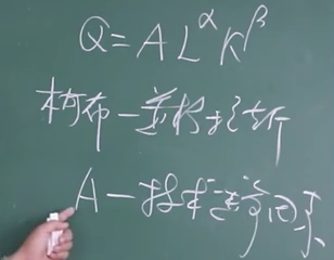
    • Besides labor and capital that can be clearly identified, the other factors are grouped into A and used to analyze how a country’s economy operates.

1.3. Fixed and Variable Factors

• Fixed factors: factors that do not change as output changes.
• Variable factors: factors that change as output changes.
• Production is divided into two types according to whether fixed factors exist:
  • Short-run production: production during a period in which at least one factor is fixed.
  • Long-run production: production during a period in which all factors are variable.

2. Short-Run Production Analysis

2.1. What It Is

• Q = f(L, K0)
  • Assume capital is fixed and only the labor factor is considered.
  • This is short-run production.
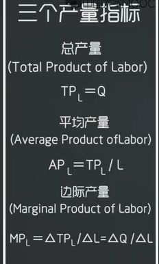
• Three output indicators
  • 

2.2. How to Analyze It

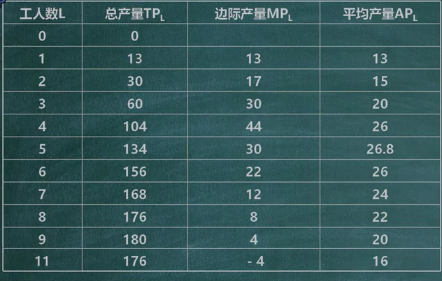
• Table method:
  • 
• Graphical method:
  • 
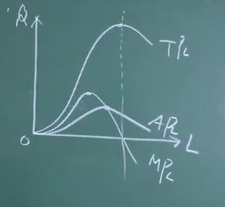
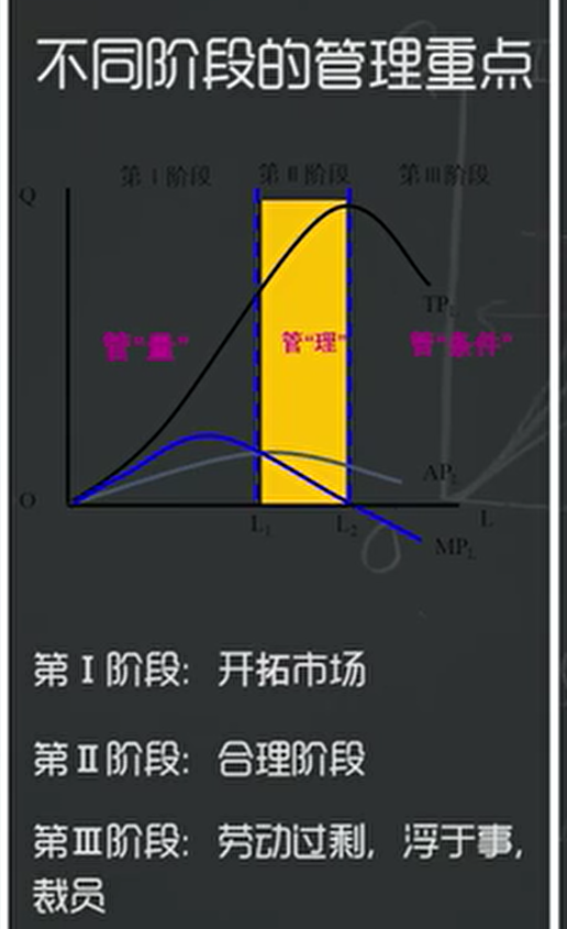
  • All three curves have a highest point.
  • When marginal product = 0, total product is at its maximum.
    • Because total product is the sum of marginal products.
  • When the marginal-product curve and average-product curve intersect, marginal product = average product, and average product is at its maximum.
• Law of diminishing marginal product
  • With other conditions unchanged, if the amount of one variable factor alone is increased, output initially grows at an increasing rate, then grows at a decreasing rate, and if the use of that factor continues to increase, output eventually decreases in absolute terms.

2.3. Use

2.3.1. Rational Stage of Production

• 

3. Long-Run Production Decisions

3.1. What It Is

• Q = f(L, K)
  • Both L and K are variable.
  • Long-run production.

3.2. How to Analyze It

3.2.1. Isoquant

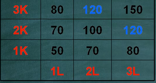
• The locus of combinations of two factors that can produce the same output.
• Table method
  • 
• Graphical method
  • 
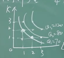
    • There are infinitely many isoquants; the higher the position, the higher the output level.
    • No two isoquants can intersect.
    • They are convex toward the origin.

3.2.2. Isocost Line

• With cost fixed, the locus of the maximum combinations of two factors that a firm can purchase.
  • 
    • 
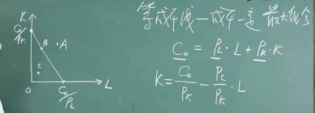
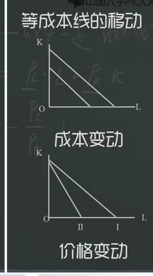
      • When cost changes, the isocost line shifts in parallel.
      • When prices change, the isocost line rotates.

3.3. Use

3.3.1. Rational Region of Production

3.3.1.1. Marginal Rate of Substitution

3.3.1.1.1. What It Is

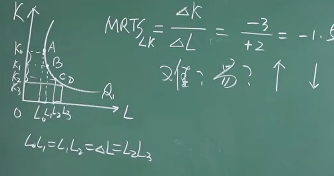
• Factors of production can substitute for one another; this is used to measure how easy the substitution is.
• Diminishing marginal rate of technical substitution
  • 

3.3.1.2. Conclusion

• 
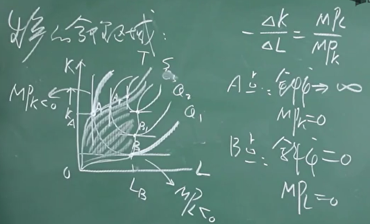
  • Draw one tangent to the isoquant parallel to L and another tangent parallel to K.
  • Going beyond the outer boundary means entering the third stage of production, which should be avoided, so production should take place within the inner region – the rational region of production.

3.3.2. Optimal Production Decision

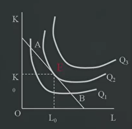
• With cost fixed, make the output decision (maximize output).
  • 
• With output fixed, make the cost decision (minimize cost).
  • 
• Decide cost and output at the same time (minimize cost and maximize output).
  • 

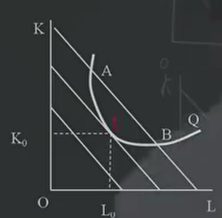
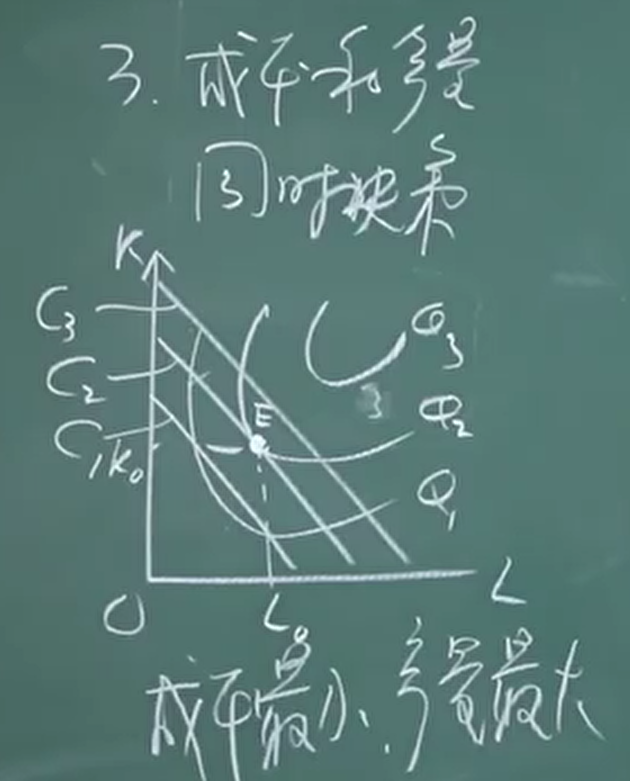
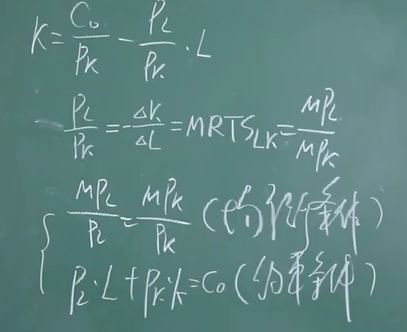
3.3.2.1. Producer Equilibrium

• The state in which producer equilibrium is reached.
  • 

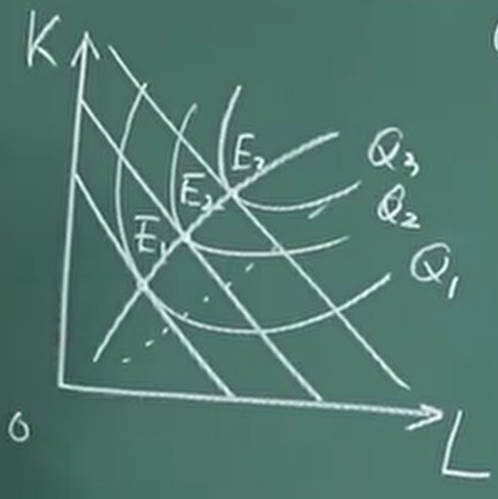
3.3.2.2. Expansion Path

3.3.2.2.1. What It Is

• The expansion path is the locus of producer-equilibrium points.
  • 

3.3.2.2.2. Use

• Used to classify types of technology.
  • 

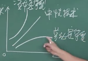
3.3.2.2.3. Expansion-Path Equation

• 
• Transformation
  • 
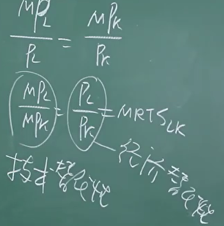
  • Explains why some countries are labor-intensive while others are capital-intensive.

4. Returns to Scale

4.1. What It Is

• The characteristics of how output changes when all factors in a production process increase by the same multiple.

4.2. Three Forms

• 
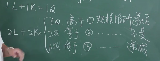
  • Increasing returns to scale
  • Constant returns to scale
  • Decreasing returns to scale
• Why returns to scale increase
  • Specialization of production
  • Specialization of management
  • Geometric factors (heavy industry)
  • Convenience conditions
• Why returns to scale are constant
  • The factors that produce increasing returns have been fully absorbed, and production is constrained by some technology.
• Why returns to scale decrease
  • Management efficiency declines.