Supply and Demand

1. Demand

1.1. What It Is

• Demand is the quantity of a good that consumers are willing and able to buy during a given period at a given price level.
  • Willing to buy: desire; potential demand.
  • Able to buy: money.
  • Demand = desire + money.
    • If only desire is satisfied, it is potential demand.
    • If both are satisfied, it is effective demand.
    • The benefit of distinguishing effective demand from potential demand: understand the actual amount of market demand.
      • For example, China has a large population but smaller effective demand, while the United States has a smaller population but larger effective demand.

1.2. Factors Affecting Demand

1.2.1. The Price of the Good Itself

• Price rises, quantity demanded falls.

1.2.2. Income Level

• Income rises, demand rises – normal goods.
• Income rises, demand falls – inferior goods.

1.2.3. Degree of Preference

1.2.4. Prices of Related Goods

• Price of good A rises, demand for B falls – complements -> firms are in a cooperative relationship.
• Price of good A rises, demand for B rises – substitutes -> firms are in a competitive relationship.
• Price of good A rises, demand for B remains unchanged – independent goods.

1.2.5. Expectations About the Future

• Good expectations for the future, demand rises.
• Poor expectations for the future, demand falls.

1.3. Effect of Price on Demand

1.3.1. Law of Demand

• Among the factors affecting demand, consider only the price of the good itself.
• Verbal description
  • Other things being equal, the quantity consumers demand of a good changes inversely with the price of the good itself.
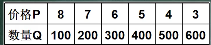
• Demand schedule
  • 
• Demand curve
  • 
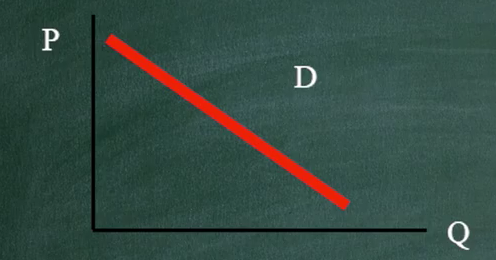
  • It represents consumers’ quantity demanded during a given period.
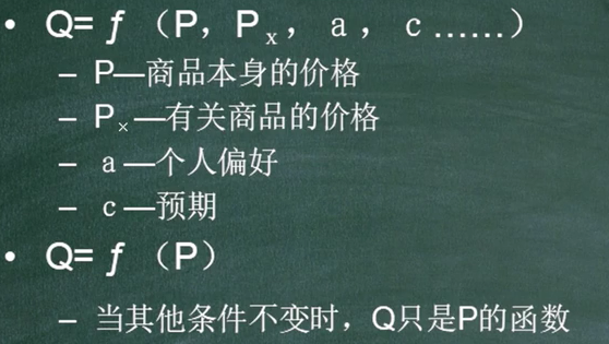
• Demand function
  • 

1.3.1.1. Market Demand

• Market demand = sum of individual demand.
• Therefore market demand also follows the law of demand.

1.3.2. Exceptions to the Law of Demand

• Price remains unchanged while demand keeps increasing.
  • 
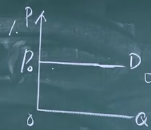
  • For example, scarce materials such as gold.
• Demand does not change no matter how high the price becomes.
  • 
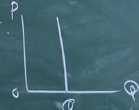
  • Necessities, such as salt and medicine.
• Price rises, demand rises.
  • 
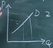
  • Non-necessities, such as luxury goods.
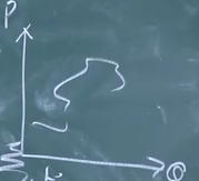
• Price rises, demand may decrease or increase.
  • 

1.4. Effects of Other Factors on Demand

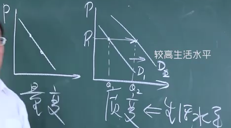
• Change in quantity demanded: a change caused by a change in price itself – quantitative change.
• Change in demand: a change caused by non-price factors – qualitative change.
• 

2. Supply

2.1. What It Is

• Supply is the quantity of a good that producers are willing and able to provide during a given period at a given price level.
  • A given period.
  • Willing to sell: willingness to sell, related to price.
  • Able to sell: output.
• Supply = willingness to sell + output -> price + output.
  • When both conditions are met, it is called effective supply (supply that has been realized).
  • When only one condition is met, it is called potential supply (supply that has not been realized).
  • The purpose of distinguishing effective supply from potential supply:
    • Measure producers’ actual income.

2.2. Factors Affecting Supply

• The price of the good itself
  • Price rises, output rises.
• Product cost
  • Cost rises, output falls.
• Technology level
  • Technology improves, output rises.
  • Productivity = (labor + capital + land) * technology.
• Prices of related goods
  • Prices of related goods rise, output falls.
• Producers’ objectives
  • Mainly the following three objectives:
    • Profit maximization.
    • Total output maximization.
    • Average output maximization.
• Future expectations
  • Good expectations for the future economy, output rises.

2.3. Effect of Price on Supply

2.3.1. Law of Supply

• Verbal description
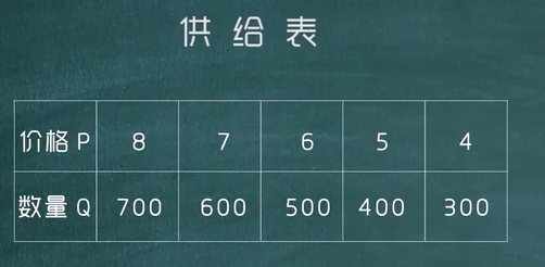
  • Other things being equal, the quantity supplied of a good changes in the same direction as the price of the good itself.
• Supply schedule
  • 
• Supply curve
  • 
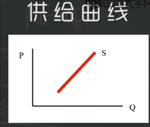
  • It applies to a given period, not to a single point in time.
• Supply function
  • Supply = f(price, prices of other goods, cost, technology).

2.3.1.1. Market Supply

• Market supply = sum of individual supply.
• Therefore market supply also follows the law of supply.

2.3.2. Exceptions to the Law of Supply

• Price remains unchanged while supply keeps increasing.
  • 
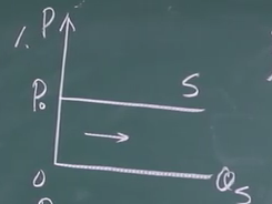
  • Beverages.
  • Some public products/services: subway, bus, tap water, etc.
• Price keeps increasing while supply remains unchanged.
  • 
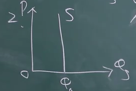
  • Antiques, land, etc.
• The lower the price, the greater the supply.
  • 
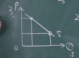
  • Assembly-line work.
• Price rises, supply may rise or fall.
  • 
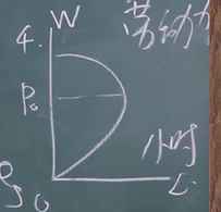
  • Wages.

2.4. Effects of Other Factors on Supply

• Change in quantity supplied: a change caused by a change in price itself – quantitative change.
• Change in supply: a change caused by non-price factors – qualitative change.
  • 

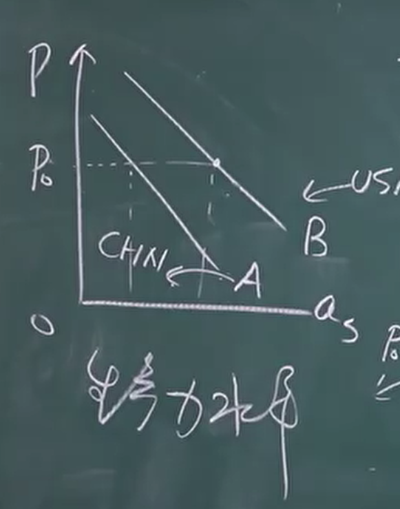
3. Market Equilibrium

• Verbal description
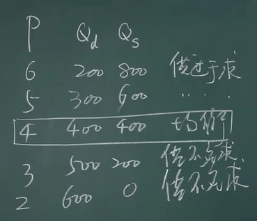
  • A market composed of demand and supply mainly has three states:
    • Excess supply.
    • Equilibrium.
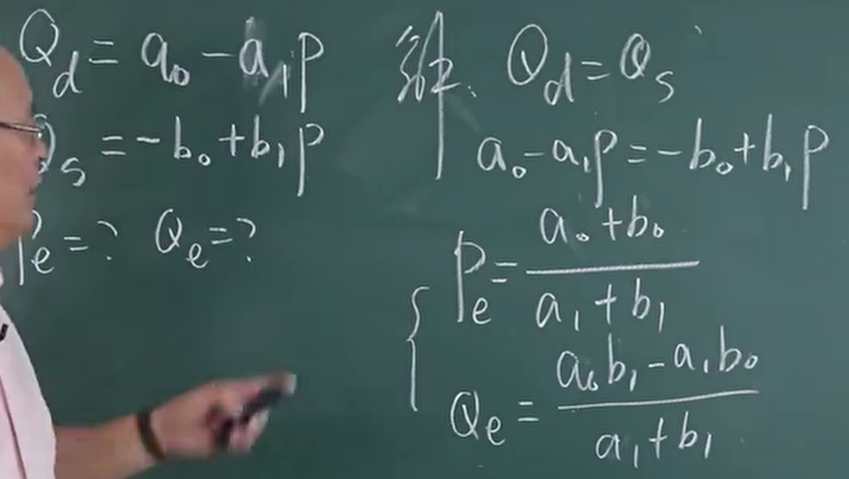
      • When demand and supply are equal, this state is called equilibrium. The price at this point is called the equilibrium price, and the quantity is called the equilibrium quantity.
    • Excess demand.
• Table method
  • 
• Graphical method
  • 
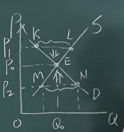
    • E is the equilibrium point.
    • K-L above E is excess supply.
    • M-N below E is excess demand.
• Formula method
  • 

3.1. Changes in Market Equilibrium

• A change in demand alone causes equilibrium price and equilibrium quantity to move in the same direction.
  • 
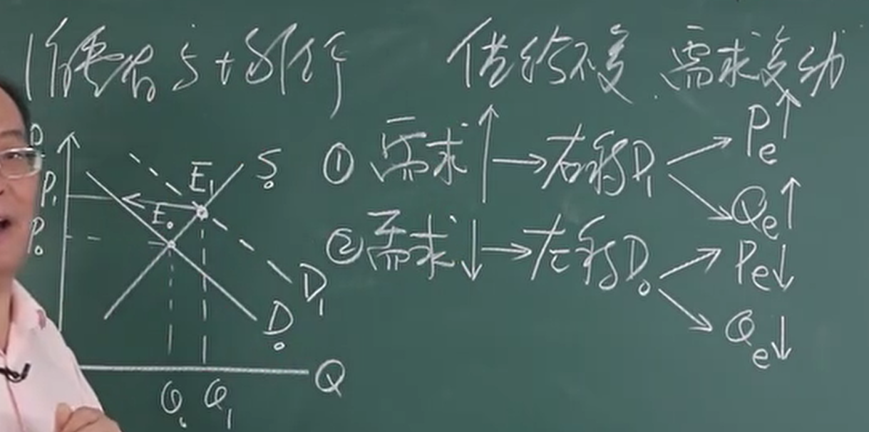
  • Demand increases, the demand curve shifts right -> equilibrium price rises, equilibrium quantity rises.
  • Demand decreases, the demand curve shifts left -> equilibrium price falls, equilibrium quantity falls.
• A change in supply alone causes equilibrium price to move in the opposite direction and equilibrium quantity to move in the same direction.
  • 
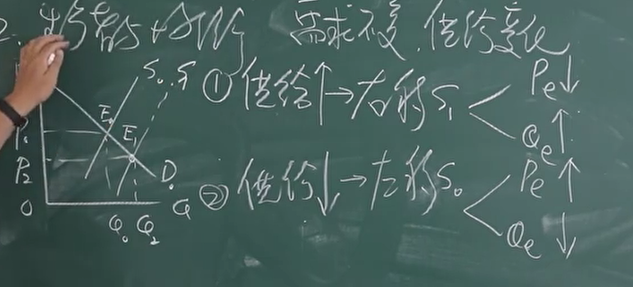
    • Supply increases, the supply curve shifts right -> equilibrium price falls, equilibrium quantity rises.
    • Supply decreases, the supply curve shifts left -> equilibrium price rises, equilibrium quantity falls.
• Simultaneous changes in demand and supply lead to more complicated changes in equilibrium.
  • 
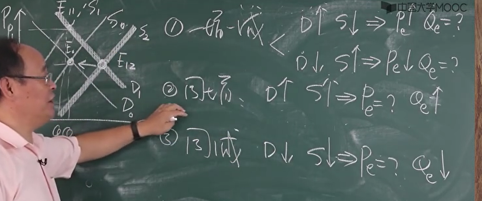
    • One increases and the other decreases.
      • Supply increases, demand decreases -> equilibrium price falls, equilibrium quantity is unknown.
      • Supply decreases, demand increases -> equilibrium price rises, equilibrium quantity is unknown.
    • Both increase.
      • Supply increases, demand increases -> equilibrium price is unknown, equilibrium quantity rises.
    • Both decrease.
      • Supply decreases, demand decreases -> equilibrium price is unknown, equilibrium quantity falls.

3.2. Price Floors and Price Ceilings

• Price floor: a minimum price above the equilibrium price.
  • 
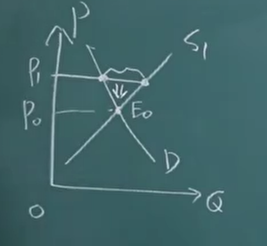
  • Excess supply; the government purchases the surplus.
  • For example, agricultural products.
• Price ceiling: a maximum price below the equilibrium price.
  • 
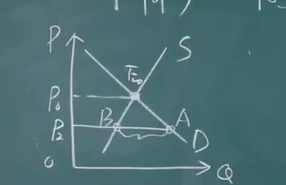
  • Excess demand; black markets and similar phenomena may appear.
  • For example, scarce goods.

3.3. Government Taxes

• Consumer surplus and producer surplus
  • 
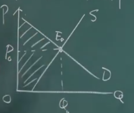
  • Consumer surplus: the benefit consumers obtain from the market; that is, P P0 E0 in the figure.
  • Producer surplus: the benefit producers obtain from the market; that is, O P0 E0 in the figure.
• Tax (using a per-unit tax on producers as the example) -> production cost rises -> the supply curve shifts left.
  • 
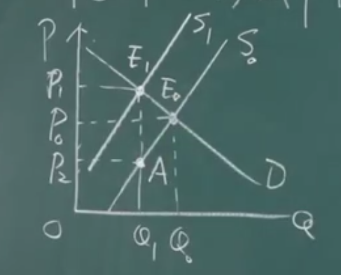
    • P1P2 = P0P1 + 0P2.
      • P1P2 is the per-unit product tax.
      • P0P1 is the consumer tax burden.
      • P0P2 is the producer tax burden.
      • Producers transfer part of the tax burden to consumers by raising prices.
    • Total loss = producer loss + consumer loss.
      • P0 P2 A E0 is producer loss.
      • P0 P1 E1 E0 is consumer loss.
    • Total benefit < total loss.
      • P1 E1 A P2 is total benefit.

3.4. Government Subsidies

• Subsidy (using a producer subsidy as the example) -> production cost falls -> the supply curve shifts right.
  • 
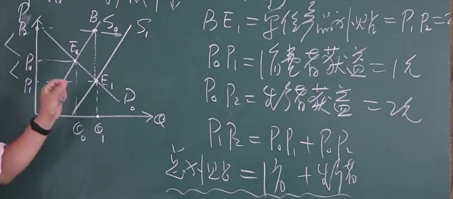
    • BE1 = P1P2 = P2P0 + P0P1.
      • BE1 is the government subsidy.
      • P0P2 is the consumer benefit.
      • P0P1 is the producer benefit.
    • Total benefit = producer benefit + consumer benefit.
      • P2 B E0 P0 is producer benefit.
      • P0 E0 E1 P1 is consumer benefit.
    • Total benefit < total expenditure.
      • P2 B E1 P1 is total expenditure.